Setting the Chromatographic Conditions

This example uses the following chromatographic conditions (the detector settings are shown in Detector settings for emission scan).

**Table:** Chromatographic Conditions
Mobile phases	A = water = 50 % B = Acetonitrile = 50 %
Column	Vydac-C18-PNA, 250 mm x 2.1 mm i.d. with 5 µm particles
Sample	PAH 0.5 ng
Flow rate	0.4 ml/min
Compressibility A (water)	46
Compressibility B (Acetonitrile)	115
Stroke A and B	auto
Time Table	at 0 min % B=50
	at 3 min % B=60
	at 14.5 min % B=90
	at 22.5 min % B=95
Stop time	26 min
Post time	8 min
Injection volume	1 µl
Oven temperature (1200)	30 °C
FLD PMT Gain	PMT = 15
FLD Response time	4 s

Figure: Detector settings for emission scan

Wait until the baseline stabilizes. Complete the run.
Load the signal. (In this example just the time range of 13 min is displayed).

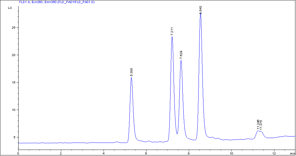
Figure: Chromatogram from Emissions Scan
Use the isoabsorbance plot and evaluate the optimal emission wavelengths, shown in the table below.

Figure: Isoabsorbance Plot from Emission Scan

Peak #
Time
Emission Wavelength
1

5.3 min

330 nm

2

7.2 min

330 nm

3

7.6 min

310 nm

4

8.6 min

360 nm

5

10.6 min

445 nm

6

11.23 min

385 nm
Using the settings and the timetable (from previous page), do a second run for the evaluation of the optimal excitation wavelength.

Figure: Detector settings for excitation scan
Wait until the baseline stabilizes. Start the run.
Load the signal.

Figure: Chromatogram - Excitation Scan at Reference Wavelength 260/330 nm

Use the isoabsorbance plot and evaluate the optimal excitation wavelengths (in this example just in the time range of 13 minutes).

Peak #	Time	Emission Wavelength	Excitation Wavelength
1	5.3 min	330 nm	220 / 280 nm
2	7.3 min	330 nm	225 / 285 nm
3	7.7 min	310 nm	265 nm
4	8.5 min	360 nm	245 nm
5	10.7 min	445 nm	280 nm
6	11.3 min	385 nm	270 / 330 nm

21-Jun-2025